We decided to use 3 datasets from the Centers for Disease Control and Prevention website (https://wwwn.cdc.gov/nchs/nhanes/search/datapage.aspx?Component=Demographics&Cycle=2021-2023). The data were collected by National Health and Nutrition Examination Survey (NHANES) from Aug 2021 to Aug 2023. The 3 datasets are: Demographic Variables and Sample Weights dataset from Demographics data, Body Measures dataset from Examination Data, and Hepatitis A dataset from Laboratory Data. All 3 datasets were published in Sep 2024 and can be found on the Centers for Disease Control and Prevention website. We will join the 3 datasets together for our project.
The specific information for the 3 datasets are the following:
2.1.0.1 Demographic Variables and Sample Weights dataset
link to data description file: https://wwwn.cdc.gov/Nchs/Nhanes/2021-2022/DEMO_L.htm
file type: XPT file
data introduction: Demographic households information by interviews and examination procedures.
dimensions: 11933 rows, 27 columns
features: Respondent sequence number, Data release cycle, Interview examination status, Gender, Age in years at screening, Age in months at screening - 0 to 24 mos, Race/Hispanic origin, Race/Hispanic origin w/ NH Asian, Six-month time period, Age in months at exam - 0 to 19 years, Served active duty in US Armed Forces, Country of birth, Length of time in US, Education level - Adults 20+, Marital status, Pregnancy status at exam, Total number of people in the Household, HH ref person’s gender, HH ref person’s age in years, HH ref person’s education level, HH ref person’s marital status, HH ref person’s spouse’s education level, Full sample 2-year interview weight, Full sample 2-year MEC exam weight, Masked variance pseudo-stratum, Masked variance pseudo-PSU, Ratio of family income to poverty
potential problems: some of the feature may hold similar information, some features may be useless, which all need to be taken care of.
2.1.0.2 Body Measures dataset
link to data description file: https://wwwn.cdc.gov/Nchs/Nhanes/2021-2022/BMX_L.htm
file type: XPT file
data introduction: Body measures information by examinations to relate between body weights and health conditions in US population.
dimensions: 8860 rows, 22 columns
features: Respondent sequence number, Body Measures Component Status Code, Weight (kg), Weight Comment, Recumbent Length (cm), Recumbent Length Comment, Head Circumference (cm), Head Circumference Comment, Standing Height (cm), Standing Height Comment, Body Mass Index (kg/m**2), BMI Category - Children/Youth, Upper Leg Length (cm), Upper Leg Length Comment, Upper Arm Length (cm), Upper Arm Length Comment, Arm Circumference (cm), Arm Circumference Comment, Waist Circumference (cm), Waist Circumference Comment, Hip Circumference (cm), Hip Circumference Comment
potential problems: contains many comments feature which may not be useful; some of the features are only present in younger population, which also need some data engineering to handle this problem
2.1.0.3 Hepatitis A dataset
link to data description file: https://wwwn.cdc.gov/Nchs/Nhanes/2021-2022/HEPA_L.htm
file type: XPT file
data introduction: Testing information in a representative sample of US population for Hepatitis prevalence estimations and prevention.
dimensions: 8611 rows, 3 columns
features: Respondent sequence number, Phlebotomy 2 Year Weight, Hepatitis A antibody
2.2 Missing value analysis
We first import the xpt data files
Code
library(haven)library(tidyverse)
── Attaching core tidyverse packages ──────────────────────── tidyverse 2.0.0 ──
✔ dplyr     1.1.4     ✔ readr     2.1.5
✔ forcats   1.0.0     ✔ stringr   1.5.1
✔ ggplot2   3.5.1     ✔ tibble    3.2.1
✔ lubridate 1.9.3     ✔ tidyr     1.3.1
✔ purrr     1.0.2
── Conflicts ────────────────────────────────────────── tidyverse_conflicts() ──
✖ dplyr::filter() masks stats::filter()
✖ dplyr::lag()    masks stats::lag()
ℹ Use the conflicted package (<http://conflicted.r-lib.org/>) to force all conflicts to become errors
Code
library(naniar)demo_data <-read_xpt("data/DEMO_L.XPT")bmx_data <-read_xpt("data/BMX_L.XPT")hep_data <-read_xpt("data/HEPA_L.XPT")combined_data <- hep_data |>left_join(bmx_data, by ="SEQN") |>left_join(demo_data, by ="SEQN")
To visualize missing values, we can make 2 graphs showing number and percentage of missing values for each features respectively.
Code
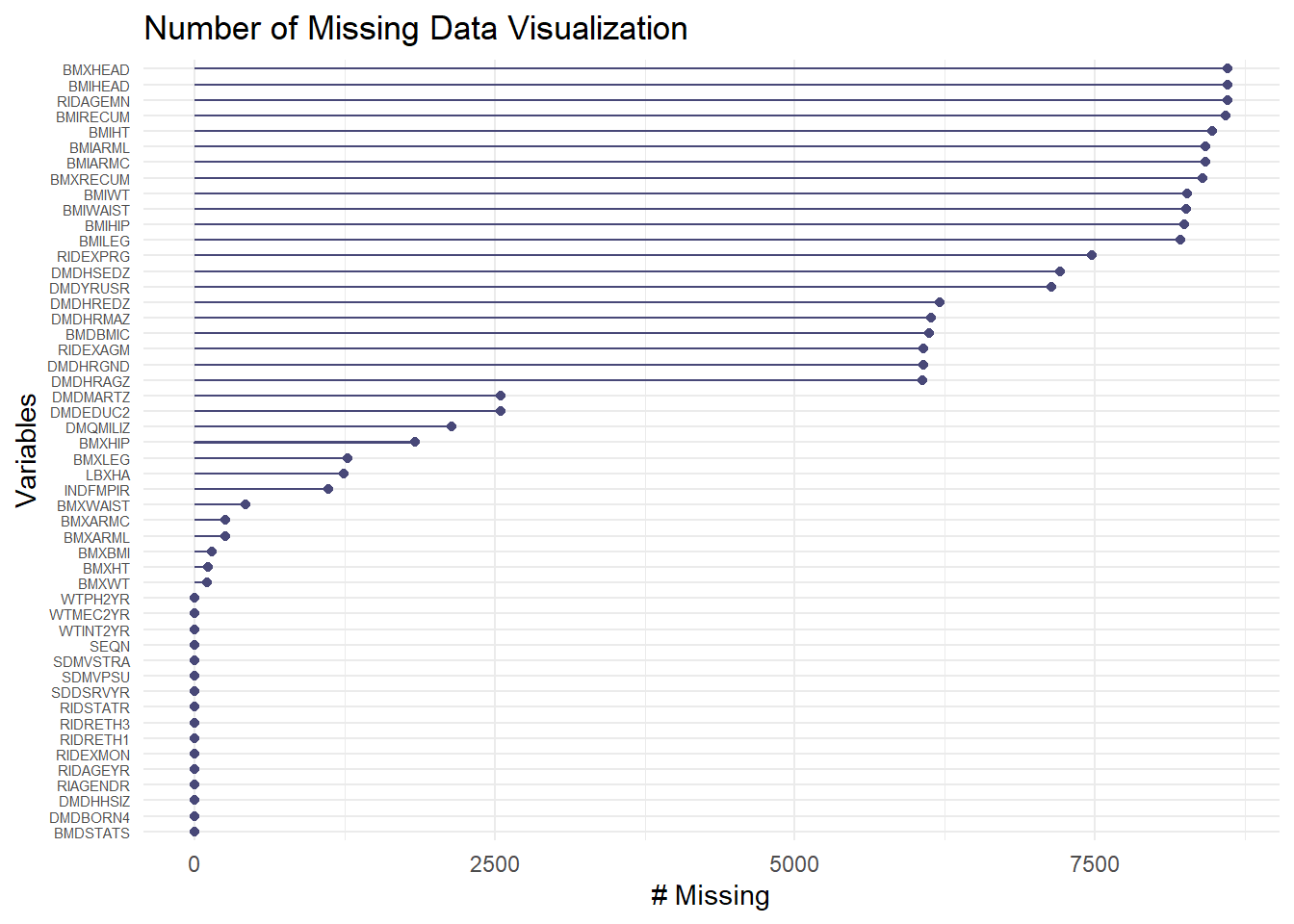
gg_miss_var(combined_data) +labs(title ="Number of Missing Data Visualization") +theme(axis.text.y =element_text(size =5.5))
From this graph, we can see that the variables with most missing values (BMXHEAD, BMIHEAD) have more than 8000 missing values, which means that almost the entire feature could be missing. On the other hand, there are also features with extremely low number of missing values like WTPH2YR, WTMEC2YR, etc. Almost no missing values within those variables. However, we also need another graph to see the percentage of missing values in each of the variables.
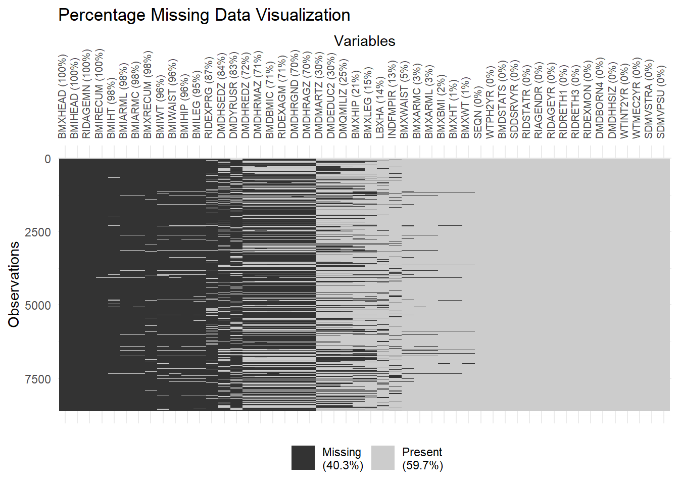
The vis_miss graph can show us the percentage of missing values both in each feature and in the entire dataset, as well as which observation is missing. From the graph, we can see that there are 4 features that are entirely missing, and 16 features with no missing values. On the scope of the entire dataset, there are 40.% of missing values in total.